2. Results - Prediction skill of Metabolic Index and its application to fish catch prediction

Results

Metabolic Index prediction skill 

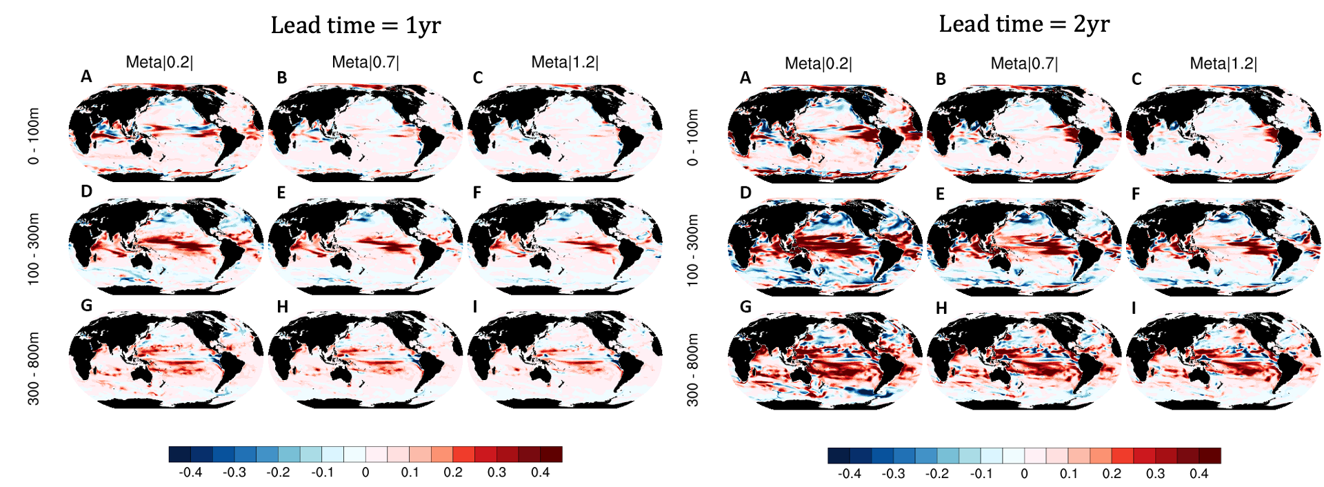
Figure 1. Predictability of metabolic index. (A-C) Prediction skill of the normalized metabolic index at 0-100 m depth, with values of (A) 0.2, (B), 0.7, and (C) 1.2. (D-F) and (G-I) are similar to (A-C), but at 100-300 m and 300-800 m depth, respectively. The prediction skill is measured by the mean annual anomaly correlation coefficient between reanalyzed data and lead-time forecasts during 1991-2017. Black dots denote statistically significant values at the 95% confidence level.

• The predictive skill of the metabolic index shows significant skill in many ocean regions in one year advance.
• The skillful prediction of the metabolic index extends to a 2-year lead time across many global oceans, particularly within the subsurface layers. Nevertheless, the predictive skill is generally reduced compared to that of a 1-year lead time.
• The notable decrease in predictive skill above the 300 m depth appears in the tropical Pacific. This limited skill is attributed to the inherent challenges dynamic models encounter in predicting interannual climate variability, such as El Niño-Southern Oscillation (ENSO), beyond a one-year horizon.

 

Prediction skill difference (Metabolic index – Temperature)

Figure 2. Differences in prediction skill between the metabolic index and temperature. (A-C) Differences in prediction skill between the normalized metabolic index and temperature at 0-100m, with values of (A) 0.2, (B), 0.7, and (C) 1.2. (D-F) and (G-I) are similar to (A-C), but at 100-300 m and 300-800 m depth, respectively. The prediction skill is measured by the mean annual anomaly correlation coefficient between reanalyzed data and lead-time forecasts during 1991-2017. Positive values indicate that the oxygen prediction skill is higher than that of temperature.

• Differences in the correlation between ECDA-COBALT and forecast for MI and T
• The higher “MI – Temp” -> better oxygen predictability than temperature predictability.
• The positive difference in prediction skill, indicating an increased predictive benefit due to oxygen, appears primarily in the tropical Pacific region.

 

Subsurface oxygen and temperature budget analysis over the tropical region 

Figure 3. Subsurface oxygen and temperature budget analysis and the persistency of the advection terms over the tropical region. Timeseries of reanalyzed subsurface (100-300m) (A) oxygen and (B) temperature advection over the tropical region (150°E-90°W,20°S-20°N) for 1991-2017. Red lines show the lateral advections which are the sum of anomalous zonal and meridional advections. Blue lines indicate the anomalous vertical advections. Black, purple, and yellow lines indicate the anomalous time tendencies, the sum of lateral and vertical advections, and the residual, respectively. The numbers in the brackets denote the correlation coefficient between the time tendency term and each term. Asterisks mean statistically significant at the 95% confidence level. Persistency of the advections in subsurface (C) oxygen and (D) temperature. Red and blue bars indicate the persistency of the lateral and the vertical advection terms, respectively. Significance at 95% level confidence is indicated by black dashed lines.

• The oxygen budget analysis indicates that the lateral advection is responsible for the oxygen anomalies over the tropical region, whereas the temperature is strongly influenced by vertical advection.
• The persistence of lateral oxygen advection which controls the temporal oxygen variability is larger than the temperature advections, suggesting that the oxygen reveals a longer memory than the temperature.
• The difference in the main drivers of oxygen and temperature variability arises from distinct characteristics in the spatial patterns of their climatology. The areas of higher predictability of oxygen relative to temperature are located along the periphery of the oxygen minimum zone (OMZ) in the eastern Pacific, defined by deficient oxygen concentrations (< 20-45 mmol kg-1).
• Horizontal inflow across the strong horizontal gradient of oxygen concentration plays a dominant role in influencing oxygen variations compared to vertical advection. In contrast to the oxygen, interannual variability of temperature in the tropical Pacific is primarily affected by the vertical fluctuations in thermocline depth, largely caused by phenomena like the ENSO.

 

Application of Metabolic Index to predict bigeye tuna

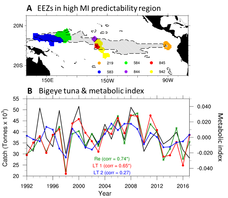
Figure 4. Predictability of Bigeye tuna using metabolic index in the tropical area where oxygen is well predicted. (A) Hatched area is a region where oxygen is well predicted, which means the difference between Metabolic Index and temperature predictability of more than 0.25. In the hatched area, the six EEZs were selected. The EEZs include Galapagos Islands (219), Kiribati (942), Palmyra Atoll & Kingman Reef (844), Jarvis Islands (845), Marshall Islands (584), and Micronesia (583). (B) Black line shows detrended reported annual catches of Bigeye tuna in EEZs where oxygen is well predicted. Green, red, and blue lines indicate the reanalyzed, the 1-year lead-time, and 2-year lead-time forecasts of Metabolic Index, respectively. Asterisks denote the significant (P < 0.05) correlation between reported catches and metabolic indexes.

• The Bigeye tuna catch was detrended to lessen the potential human error of fishing effort trends onto environmental elements.
• Metabolic index was applied to predict bigeye. Bigeye tuna catches could be predicted for up to one year using the Metabolic Index.